The RAM-OP Workflow is summarised in the diagram below.
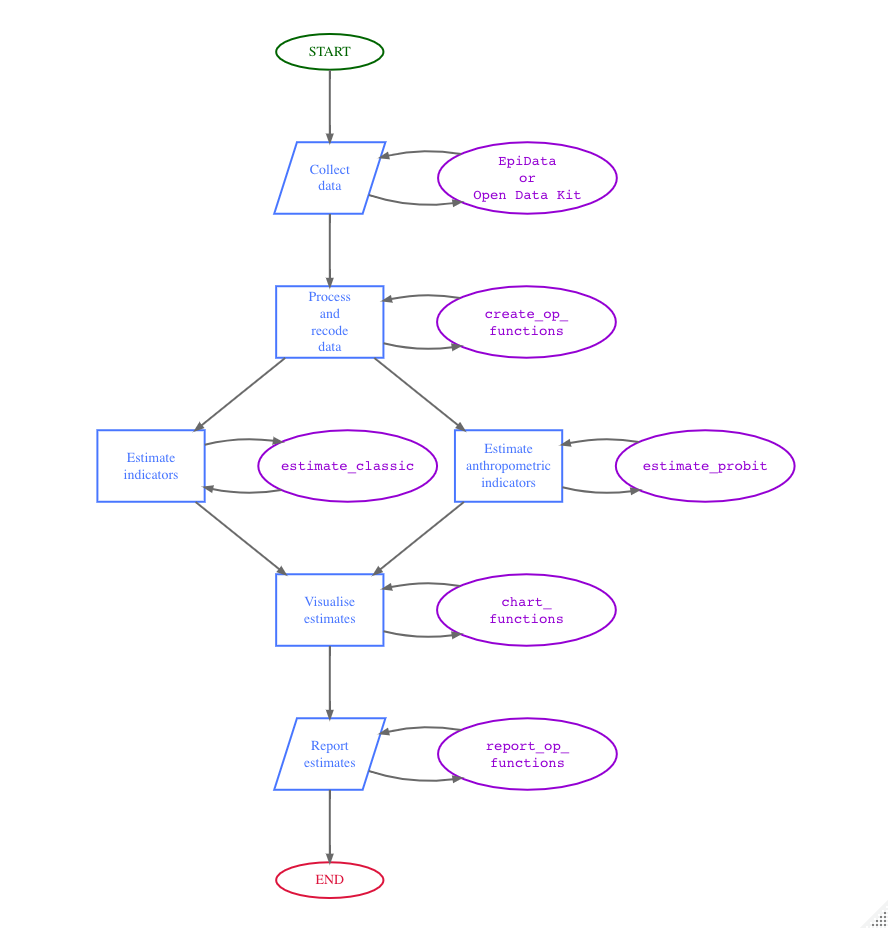
The oldr package provides functions to use for all steps
after data collection. These functions were developed specifically for
the data structure created by the EpiData
or the Open Data
Kit collection tools. The data structure produced by these
collection tools is shown by the dataset testSVY included
in the oldr package.
testSVY
#> # A tibble: 192 × 90
#>      ad2   psu    hh    id    d1    d2    d3    d4    d5    f1   f2a   f2b   f2c
#>    <int> <int> <int> <int> <int> <int> <int> <int> <int> <int> <int> <int> <int>
#>  1     1   201     1     1     1    67     2     5     2     3     2     1     1
#>  2     1   201     2     1     1    74     1     2     2     3     2     1     1
#>  3     1   201     3     1     1    60     1     2     2     2     2     2     2
#>  4     1   201     3     2     1    60     2     2     2     3     2     2     1
#>  5     1   201     4     1     1    85     2     5     2     3     2     1     1
#>  6     1   201     5     1     2    86     1     5     1     4     2     1     1
#>  7     1   201     6     1     1    80     1     5     2     3     2     1     1
#>  8     1   201     6     2     1    60     2     5     2     3     2     2     1
#>  9     1   201     7     1     1    62     1     2     2     2     2     1     1
#> 10     1   201     8     1     1    72     2     5     2     2     2     1     1
#> # ℹ 182 more rows
#> # ℹ 77 more variables: f2d <int>, f2e <int>, f2f <int>, f2g <int>, f2h <int>,
#> #   f2i <int>, f2j <int>, f2k <int>, f2l <int>, f2m <int>, f2n <int>,
#> #   f2o <int>, f2p <int>, f2q <int>, f2r <int>, f2s <int>, f3 <int>, f4 <int>,
#> #   f5 <int>, f6 <int>, f7 <int>, a1 <int>, a2 <int>, a3 <int>, a4 <int>,
#> #   a5 <int>, a6 <int>, a7 <int>, a8 <int>, k6a <int>, k6b <int>, k6c <int>,
#> #   k6d <int>, k6e <int>, k6f <int>, ds1 <int>, ds2 <int>, ds3 <int>, …
Processing and recoding data
Once RAM-OP data is collected, it will need to be processed and
recoded based on the definitions of the various indicators included in
RAM-OP. The oldr package provides a suite functions to
perform this processing and recoding. These functions and their syntax
can be easily remembered as the create_op_ functions as
their function names start with the create_ verb followed
by the op_ label and then followed by an indicator or
indicator set specific identifier or short name. Finally, an additional
tag for male or female can be added to the
main function to provide gender-specific outputs.
Currently, a standard RAM-OP can provide results for the 13 indicators or indicator sets for older people. The following table shows these indicators/indicator sets alongside the functions related to them:
| Indicator / Indicator Set | Related Functions |
|---|---|
| Demography and situation |
create_op_demo;
create_op_demo_males;
create_op_demo_females
|
| Food intake |
create_op_food;
create_op_food_males;
create_op_food_females
|
| Severe food insecurity |
create_op_hunger;
create_op_hunger_males;
create_op_hunger_females
|
| Disability |
create_op_disability;
create_op_disability_males;
create_op_disability_females
|
| Activities of daily living |
create_op_adl;
create_op_adl_males;
create_op_adl_females
|
| Mental health and well-being |
create_op_mental;
create_op_mental_males;
create_op_mental_females
|
| Dementia |
create_op_dementia;
create_op_dementia_males;
create_op_dementia_females
|
| Health and health-seeking behaviour |
create_op_health;
create_op_health_males;
create_op_health_females
|
| Sources of income |
create_op_income;
create_op_income_males;
create_op_income_females
|
| Water, sanitation, and hygiene |
create_op_wash;
create_op_wash_males;
create_op_wash_females
|
| Anthropometry and anthropometric screening coverage |
create_op_anthro;
create_op_anthro_males;
create_op_anthro_females
|
| Visual impairment |
create_op_visual;
create_op_visual_males;
create_op_visual_females
|
| Miscellaneous |
create_op_misc;
create_op_misc_males;
create_op_misc_females
|
A final function in the processing and recoding set -
create_op - is provided to perform the processing and
recoding of all indicators or indicator sets. This function allows for
the specification of which indicators or indicator sets to process and
recode which is useful for cases where not all the indicators or
indicator sets have been collected or if only specific indicators or
indicator sets need to be analysed or reported. This function also
specifies whether a specific gender subset of the data is needed.
For a standard RAM-OP implementation, this step is performed in R as follows:
## Process and recode all standard RAM-OP indicators in the testSVY dataset
create_op(svy = testSVY)
which results in the following output:
#> # A tibble: 192 × 138
#>      psu  sex1  sex2 resp1 resp2 resp3 resp4   age ageGrp1 ageGrp2 ageGrp3
#>    <int> <dbl> <dbl> <dbl> <dbl> <dbl> <dbl> <int>   <dbl>   <dbl>   <dbl>
#>  1   201     0     1     1     0     0     0    67       0       1       0
#>  2   201     1     0     1     0     0     0    74       0       0       1
#>  3   201     1     0     1     0     0     0    60       0       1       0
#>  4   201     0     1     1     0     0     0    60       0       1       0
#>  5   201     0     1     1     0     0     0    85       0       0       0
#>  6   201     1     0     0     1     0     0    86       0       0       0
#>  7   201     1     0     1     0     0     0    80       0       0       0
#>  8   201     0     1     1     0     0     0    60       0       1       0
#>  9   201     1     0     1     0     0     0    62       0       1       0
#> 10   201     0     1     1     0     0     0    72       0       0       1
#> # ℹ 182 more rows
#> # ℹ 127 more variables: ageGrp4 <dbl>, ageGrp5 <dbl>, marital1 <dbl>,
#> #   marital2 <dbl>, marital3 <dbl>, marital4 <dbl>, marital5 <dbl>,
#> #   marital6 <dbl>, alone <dbl>, MF <dbl>, DDS <dbl>, FG01 <dbl>, FG02 <dbl>,
#> #   FG03 <dbl>, FG04 <dbl>, FG05 <dbl>, FG06 <dbl>, FG07 <dbl>, FG08 <dbl>,
#> #   FG09 <dbl>, FG10 <dbl>, FG11 <dbl>, proteinRich <dbl>, pProtein <dbl>,
#> #   aProtein <dbl>, pVitA <dbl>, aVitA <dbl>, xVitA <dbl>, ironRich <dbl>, …
Estimating indicators
Once data has been processed and appropriate recoding for indicators has been performed, indicator estimates can now be calculated.
It is important to note that estimation procedures need to account for the sample design. All major statistical analysis software can do this (details vary). There are two things to note:
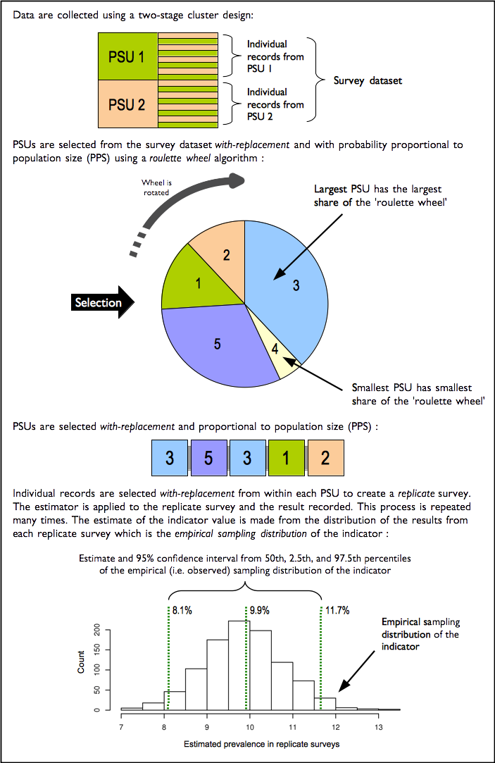
The RAM-OP sample is a two-stage sample. Subjects are sampled from a small number of primary sampling units (PSUs).
The RAM-OP sample is not prior weighted. This means that per-PSU sampling weights are needed. These are usually the populations of the PSU.
This sample design will need to be specified to statistical analysis software being used. If no weights are provided, then the analysis may produce estimates that place undue weight to observations from smaller communities with confidence intervals with lower than nominal coverage (i.e. they will be too narrow).
Blocked weighted bootstrap
The oldr package uses blocked weighted
bootstrap estimation approach:
Blocked : The block corresponds to the PSU or cluster.
Weighted : The RAM-OP sampling procedure does not use population proportional sampling to weight the sample prior to data collection as is done with SMART type surveys. This means that a posterior weighting procedure is required. The standard RAM-OP software uses a “roulette wheel” algorithm to weight (i.e. by population) the selection probability of PSUs in bootstrap replicates.
A total of m PSUs are sampled with-replacement from the
survey dataset where m is the number of PSUs in the survey
sample. Individual records within each PSU are then sampled
with-replacement. A total of n records are sampled
with-replacement from each of the selected PSUs where n is
the number of individual records in a selected PSU. The resulting
collection of records replicates the original survey in terms of both
sample design and sample size. A large number of replicate surveys are
taken (the standard RAM-OP software uses
replicate surveys but this can be changed). The required statistic
(e.g. the mean of an indicator value) is applied to each replicate
survey. The reported estimate consists of the 50th (point estimate),
2.5th (lower 95% confidence limit), and the 97.5th (upper 95% confidence
limit) percentiles of the distribution of the statistic observed across
all replicate surveys. The blocked weighted bootstrap procedure is
outlined in the figure below.
The principal advantages of using a bootstrap estimator are:
Bootstrap estimators work well with small sample sizes.
The method is non-parametric and uses empirical rather than theoretical distributions. There are no assumptions of things like normality to worry about.
The method allows estimation of the sampling distribution of almost any statistic using only simple computational methods.
PROBIT estimator
The prevalence of GAM, MAM, and SAM are estimated using a PROBIT estimator. This type of estimator provides better precision than a classic estimator at small sample sizes as discussed in the following literature:
World Health Organisation, Physical Status: The use and interpretation of anthropometry. Report of a WHO expert committee, WHO Technical Report Series 854, WHO, Geneva, 1995
Dale NM, Myatt M, Prudhon C, Briend, A, “Assessment of the PROBIT approach for estimating the prevalence of global, moderate and severe acute malnutrition from population surveys”, Public Health Nutrition, 1–6. https://doi.org/10.1017/s1368980012003345, 2012
Blanton CJ, Bilukha, OO, “The PROBIT approach in estimating the prevalence of wasting: revisiting bias and precision”, Emerging Themes in Epidemiology, 10(1), 2013, p. 8
An estimate of GAM prevalence can be made using a classic estimator:
On the other hand, the estimate of GAM prevalence made from the RAM-OP survey data is made using a PROBIT estimator. The PROBIT function is also known as the inverse cumulative distribution function. This function converts parameters of the distribution of an indicator (e.g. the mean and standard deviation of a normally distributed variable) into cumulative percentiles. This means that it is possible to use the normal PROBIT function with estimates of the mean and standard deviation of indicator values in a survey sample to predict (or estimate) the proportion of the population falling below a given threshold. For example, for data with a mean MUAC of 256 mm and a standard deviation of 28 mm the output of the normal PROBIT function for a threshold of 210 mm is 0.0502 meaning that 5.02% of the population are predicted (or estimated) to fall below the 210 mm threshold.
Both the classic and the PROBIT methods can be thought of as estimating area:

The principal advantage of the PROBIT approach is that the required sample size is usually smaller than that required to estimate prevalence with a given precision using the classic method.
The PROBIT method assumes that MUAC is a normally distributed variable. If this is not the case then the distribution of MUAC is transformed towards normality.
The prevalence of SAM is estimated in a similar way to GAM. The prevalence of MAM is estimated as the difference between the GAM and SAM prevalence estimates:
Classic estimator
The function estimateClassic in oldr
implements the blocked weighted bootstrap classic estimator of RAM-OP.
This function uses the bootClassic statistic to estimate
indicator values.
The estimateClassic function is used for all the
standard RAM-OP indicators except for anthropometry. The function is
used as follows:
## Process and recode RAM-OP data (testSVY)
df <- create_op(svy = testSVY)

## Perform classic estimation on recoded data using appropriate weights provided by testPSU
classicDF <- estimate_classic(x = df, w = testPSU)
This results in (using limited replicates to reduce computing time):
#> # A tibble: 136 × 10
#>    INDICATOR EST.ALL LCL.ALL UCL.ALL EST.MALES LCL.MALES UCL.MALES EST.FEMALES
#>    <chr>       <dbl>   <dbl>   <dbl>     <dbl>     <dbl>     <dbl>       <dbl>
#>  1 resp1      0.859   0.794   0.880     0.803     0.743     0.835      0.849
#>  2 resp2      0.0885  0.075   0.152     0.1       0.0308    0.125      0.123
#>  3 resp3      0.0417  0.0219  0.0729    0.0658    0.0309    0.166      0.0169
#>  4 resp4      0       0       0.0229    0.0132    0         0.0889     0.00826
#>  5 age       70.7    69.4    72.1      71.0      69.3      72.5       71.1
#>  6 ageGrp1    0       0       0         0         0         0          0
#>  7 ageGrp2    0.536   0.441   0.586     0.470     0.423     0.609      0.517
#>  8 ageGrp3    0.229   0.181   0.328     0.325     0.211     0.380      0.218
#>  9 ageGrp4    0.198   0.123   0.277     0.153     0.0890    0.268      0.272
#> 10 ageGrp5    0.0365  0.0219  0.0573    0.0488    0.0236    0.0747     0.0391
#> # ℹ 126 more rows
#> # ℹ 2 more variables: LCL.FEMALES <dbl>, UCL.FEMALES <dbl>
PROBIT estimator
The function estimateProbit in oldr
implements the blocked weighted bootstrap PROBIT estimator of RAM-OP.
This function uses the probit_GAM and the
probit_SAM statistic to estimate indicator values.
The estimateProbit function is used for only the
anthropometric indicators. The function is used as follows:
## Process and recode RAM-OP data (testSVY)
df <- create_op(svy = testSVY)

## Perform probit estimation on recoded data using appropriate weights provided by testPSU
probitDF <- estimate_probit(x = df, w = testPSU)
This results in (using limited replicates to reduce computing time):
#> # A tibble: 3 × 10
#>   INDICATOR  EST.ALL   LCL.ALL UCL.ALL EST.MALES LCL.MALES UCL.MALES EST.FEMALES
#>   <chr>        <dbl>     <dbl>   <dbl>     <dbl>     <dbl>     <dbl>       <dbl>
#> 1 GAM       0.0366     1.37e-2 0.0479   6.02e- 3  8.33e- 4  0.0115       0.0549
#> 2 MAM       0.0326     1.36e-2 0.0478   5.84e- 3  7.71e- 4  0.0115       0.0505
#> 3 SAM       0.000219   2.07e-6 0.00659  2.19e-10  2.59e-21  0.000160     0.00255
#> # ℹ 2 more variables: LCL.FEMALES <dbl>, UCL.FEMALES <dbl>
The two sets of estimates are then merged using the
merge_op function as follows:
## Merge classicDF and probitDF
resultsDF <- merge_op(x = classicDF, y = probitDF)

resultsDF
which results in:
#> # A tibble: 139 × 13
#>    INDICATOR GROUP       LABEL TYPE  EST.ALL LCL.ALL UCL.ALL EST.MALES LCL.MALES
#>    <fct>     <fct>       <fct> <fct>   <dbl>   <dbl>   <dbl>     <dbl>     <dbl>
#>  1 resp1     Survey      Resp… Prop…  0.859   0.794   0.880     0.803     0.743
#>  2 resp2     Survey      Resp… Prop…  0.0885  0.075   0.152     0.1       0.0308
#>  3 resp3     Survey      Resp… Prop…  0.0417  0.0219  0.0729    0.0658    0.0309
#>  4 resp4     Survey      Resp… Prop…  0       0       0.0229    0.0132    0
#>  5 age       Demography… Mean… Mean  70.7    69.4    72.1      71.0      69.3
#>  6 ageGrp1   Demography… Self… Prop…  0       0       0         0         0
#>  7 ageGrp2   Demography… Self… Prop…  0.536   0.441   0.586     0.470     0.423
#>  8 ageGrp3   Demography… Self… Prop…  0.229   0.181   0.328     0.325     0.211
#>  9 ageGrp4   Demography… Self… Prop…  0.198   0.123   0.277     0.153     0.0890
#> 10 ageGrp5   Demography… Self… Prop…  0.0365  0.0219  0.0573    0.0488    0.0236
#> # ℹ 129 more rows
#> # ℹ 4 more variables: UCL.MALES <dbl>, EST.FEMALES <dbl>, LCL.FEMALES <dbl>,
#> #   UCL.FEMALES <dbl>
Creating charts
Once indicators has been estimated, the outputs can then be used to
create relevant charts to visualise the results. A set of functions that
start with the verb chart_op_ is provided followed by the
indicator identifier to specify the type of indicator to visualise. The
output of the function is a PNG file saved in the specified filename
appended to the indicator identifier within the current working
directory or saved in the specified filename appended to the indicator
identifier in the specified directory path.
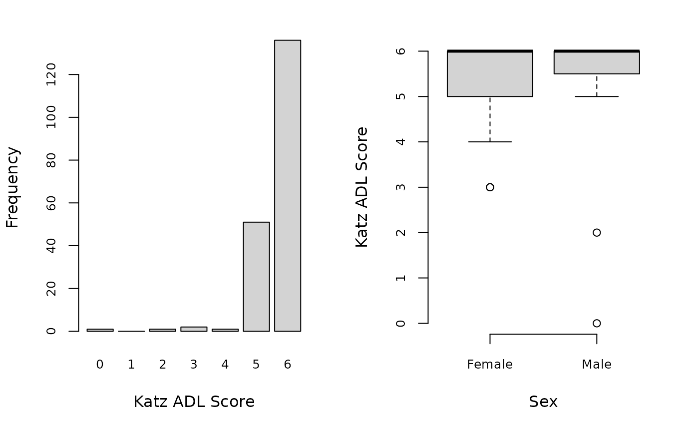
The following shows how to produce the chart for ADLs saved with filename test appended at the start inside a temporary directory:
chart_op_adl(x = create_op(testSVY), filename = file.path(tempdir(), "test"))
#> agg_png
#>       2
The resulting PNG file can be found in the temporary directory
file.exists(path = file.path(tempdir(), "test.png"))
#> [1] FALSE
and will look something like this:
Reporting estimates
Finally, estimates can be reported through report tables. The
report_op_table function facilitates this through the
following syntax:
report_op_table(estimates = resultsDF, filename = file.path(tempdir(), "TEST"))The resulting CSV file is found in the temporary directory
file.exists(path = file.path(tempdir(), "TEST.csv"))
#> [1] FALSE
and will look something like this:
#> X X.1
#> 1 Survey
#> 2
#> 3 INDICATOR TYPE
#> 4 Respondent : SUBJECT 2
#> 5 Respondent : FAMILY CARER 2
#> 6 Respondent : OTHER CARER 2
#> 7 Respondent : OTHER 2
#> 8
#> 9 Demography and situation
#> 10
#> 11 INDICATOR TYPE
#> 12 Mean self-reported age of subject (years) 1
#> 13 Self-reported age between 50 and 59 years 2
#> 14 Self-reported age between 60 and 69 years 2
#> 15 Self-reported age between 70 and 79 years 2
#> 16 Self-reported age between 80 and 89 years 2
#> 17 Self-reported age 90 years or older 2
#> 18 Sex : MALE 2
#> 19 Sex : FEMALE 2
#> 20 Marital status : SINGLE (NEVER MARRIED) 2
#> 21 Marital status : MARRIED 2
#> 22 Marital status : LIVING TOGETHER 2
#> 23 Marital status : DIVORCED 2
#> 24 Marital status : WIDOWED 2
#> 25 Marital status : OTHER 2
#> 26 Subject lives alone 2
#> 27
#> 28 Diet
#> 29
#> 30 INDICATOR TYPE
#> 31 Meal frequency (i.e. number of meals and snacks in previous 24 hours) 1
#> 32 Dietary diversity (count from 11 food groups) 1
#> 33 Consumed CEREALS (in previous 24 hours) 2
#> 34 Consumed ROOTS / TUBERS (in previous 24 hours) 2
#> 35 Consumed FRUITS / VEGETABLES (in previous 24 hours) 2
#> 36 Consumed MEAT (in previous 24 hours) 2
#> 37 Consumed EGGS (in previous 24 hours) 2
#> 38 Consumed FISH (in previous 24 hours) 2
#> 39 Consumed LEGUMES / NUTS / SEEDS (in previous 24 hours) 2
#> 40 Consumed MILK / MILK PRODUCTS (in previous 24 hours) 2
#> 41 Consumed FATS (in previous 24 hours) 2
#> 42 Consumed SUGARS (in previous 24 hours) 2
#> 43 Consumed OTHER (in previous 24 hours) 2
#> 44
#> 45 Nutrients
#> 46
#> 47 INDICATOR TYPE
#> 48 PROTEIN rich foods in diet 2
#> 49 Protein rich plant sources of protein in diet 2
#> 50 Protein rich animal sources of protein in diet 2
#> 51 Plant sources of Vitamin A in diet 2
#> 52 Animal sources of Vitamin A in diet 2
#> 53 Any source of Vitamin A 2
#> 54 IRON rich foods in diet 2
#> 55 CALCIUM rich foods in diet 2
#> 56 ZINC rich foods in diet 2
#> 57 Vitamin B1 rich foods in diet 2
#> 58 Vitamin B2 rich foods in diet 2
#> 59 Vitamin B3 rich foods in diet 2
#> 60 Vitamin B6 rich foods in diet 2
#> 61 Vitamin B12 rich foods in diet 2
#> 62 Vitamin B1 / B2 / B3 / B6 / B12 rich foods in diet 2
#> 63
#> 64 Food Security
#> 65
#> 66 INDICATOR TYPE
#> 67 Little or no hunger in household (HHS = 0 / 1) 2
#> 68 Moderate hunger in household (HHS = 2 / 3) 2
#> 69 Severe hunger in household (HHS = 4 / 5 / 6) 2
#> 70
#> 71 Disability (WG)
#> 72
#> 73 INDICATOR TYPE
#> 74 Vision : D0 : None 2
#> 75 Vision : D1 : Any 2
#> 76 Vision : D2 : Moderate or severe 2
#> 77 Vision : D3: Severe 2
#> 78 Hearing : D0 : None 2
#> 79 Hearing : D1 : Any 2
#> 80 Hearing : D2 : Moderate or severe 2
#> 81 Hearing : D3: Severe 2
#> 82 Mobility : D0 : None 2
#> 83 Mobility : D1 : Any 2
#> 84 Mobility : D2 : Moderate or severe 2
#> 85 Mobility : D3: Severe 2
#> 86 Remembering : D0 : None 2
#> 87 Remembering : D1 : Any 2
#> 88 Remembering : D2 : Moderate or severe 2
#> 89 Remembering : D3: Severe 2
#> 90 Self-care : D0 : None 2
#> 91 Self-care : D1 : Any 2
#> 92 Self-care : D2 : Moderate or severe 2
#> 93 Self-care : D3: Severe 2
#> 94 Communicating : D0 : None 2
#> 95 Communicating : D1 : Any 2
#> 96 Communicating : D2 : Moderate or severe 2
#> 97 Communicating : D3: Severe 2
#> 98 No disability in Washington Group domains 2
#> 99 At least 1 domain with any disability (P1) 2
#> 100 At least 1 domain with moderate or severe disability (P2) 2
#> 101 At least 1 domain with severe disability (P3) 2
#> 102 Multiple disability : More than one domain with any disability (PM) 2
#> 103
#> 104 Activities of daily living
#> 105
#> 106 INDICATOR TYPE
#> 107 Independent : Bathing 2
#> 108 Independent : Dressing 2
#> 109 Independent : Toileting 2
#> 110 Independent : Transferring (mobility) 2
#> 111 Independent : Continence 2
#> 112 Independent : Feeding 2
#> 113 Katz ADL score 1
#> 114 Independent (Katz ADL score = 5/6) 2
#> 115 Partial dependency (Katz ADL score = 3/4) 2
#> 116 Severe dependency (Katz ADL score = 0/1/2) 2
#> 117 Subject has someone to help them with activities of daily living 2
#> 118 Subject has ADL needs (ADL < 6) but has no helper 2
#> 119
#> 120 Mental health
#> 121
#> 122 INDICATOR TYPE
#> 123 K6 psychological distress score 1
#> 124 Serious psychological distress (K6 > 12) 2
#> 125 Probable dementia by brief CSID screen 2
#> 126
#> 127 Health
#> 128
#> 129 INDICATOR TYPE
#> 130 Long term disease requiring regular medication 2
#> 131 Takes medication for long term disease requiring regular medication 2
#> 132 Not taking drugs for long term disease : NO DRUGS AVAILABLE 2
#> 133 Not taking drugs for long term disease : TOO EXPENSIVE / NO MONEY 2
#> 134 Not taking drugs for long term disease : TOO OLD TO LOOK FOR CARE 2
#> 135 Not taking drugs for long term disease : USE OF TRADITIONAL MEDICINE 2
#> 136 Not taking drugs for long term disease : DRUGS DON'T HELP 2
#> 137 Not taking drugs for long term disease : NO-ONE TO HELP ME 2
#> 138 Not taking drugs for long term disease : NO NEED 2
#> 139 Not taking drugs for long term disease : OTHER 2
#> 140 Not taking drugs for long term disease : NO REASON GIVEN 2
#> 141 Recent illness (i.e. in the previous 2 weeks) 2
#> 142 Accessed care for recent illness 2
#> 143 Not accessing care for recent illness : NO DRUGS AVAILABLE 2
#> 144 Not accessing care for recent illness : TOO EXPENSIVE / NO MONEY 2
#> 145 Not accessing care for recent illness : TOO OLD TO LOOK FOR CARE 2
#> 146 Not accessing care for recent illness : USE OF TRADITIONAL MEDICINE 2
#> 147 Not accessing care for recent illness : DRUGS DON'T HELP 2
#> 148 Not accessing care for recent illness : NO-ONE TO HELP ME 2
#> 149 Not accessing care for recent illness : NO NEED 2
#> 150 Not accessing care for recent illness : OTHER 2
#> 151 Not accessing care for recent illness : NO REASON GIVEN 2
#> 152 Bilateral pitting oedema (may not be nutritional) 2
#> 153 Visual impairment (visual acuity < 6 / 12) by tumbling E method 2
#> 154 Problems chewing food (self-report) 2
#> 155
#> 156 Income
#> 157
#> 158 INDICATOR TYPE
#> 159 Has a personal source of income 2
#> 160 Source of income : Agriculture / fishing / livestock 2
#> 161 Source of income : Wages / salary 2
#> 162 Source of income : Sale of charcoal / bricks / etc. 2
#> 163 Source of income : Trading (e.g. market or shop) 2
#> 164 Source of income : Investments 2
#> 165 Source of income : Spending savings / sales of assets 2
#> 166 Source of income : Charity 2
#> 167 Source of income : Cash transfer / social security / welfare 2
#> 168 Source of income : Other source(s) of income 2
#> 169
#> 170 WASH
#> 171
#> 172 INDICATOR TYPE
#> 173 Improved source of drinking water 2
#> 174 Safe drinking water 2
#> 175 Improved sanitation facility 2
#> 176 Improved non-shared sanitation facility 2
#> 177
#> 178 Relief
#> 179
#> 180 INDICATOR TYPE
#> 181 Previously screened (MUAC or oedema) 2
#> 182 Anyone in household receives a ration 2
#> 183 Received non-food relief items in previous month 2
#> 184
#> 185 Anthropometry
#> 186
#> 187 INDICATOR TYPE
#> 188 Global acute malnutrition : GAM 2
#> 189 Moderate acute malnutrition : MAM 2
#> 190 Severe acute malnutrition : SAM 2
#> X.2 X.3 X.4 X.5 X.6 X.7 X.8 X.9 X.10
#> 1
#> 2 ALL MALES FEMALES
#> 3 EST LCL UCL EST LCL UCL EST LCL UCL
#> 4 0.8594 0.7938 0.8802 0.8026 0.7433 0.8345 0.8487 0.7862 0.8832
#> 5 0.0885 0.0750 0.1521 0.1000 0.0308 0.1252 0.1228 0.0874 0.1868
#> 6 0.0417 0.0219 0.0729 0.0658 0.0309 0.1662 0.0169 0.0079 0.0357
#> 7 0.0000 0.0000 0.0229 0.0132 0.0000 0.0889 0.0083 0.0000 0.0169
#> 8
#> 9
#> 10 ALL MALES FEMALES
#> 11 EST LCL UCL EST LCL UCL EST LCL UCL
#> 12 70.7396 69.4344 72.0948 71.0263 69.3453 72.5406 71.1102 70.0183 73.5077
#> 13 0.0000 0.0000 0.0000 0.0000 0.0000 0.0000 0.0000 0.0000 0.0000
#> 14 0.5365 0.4406 0.5865 0.4699 0.4235 0.6090 0.5169 0.3833 0.5868
#> 15 0.2292 0.1813 0.3281 0.3253 0.2114 0.3802 0.2185 0.1430 0.3178
#> 16 0.1979 0.1229 0.2771 0.1529 0.0890 0.2677 0.2719 0.1293 0.3135
#> 17 0.0365 0.0219 0.0573 0.0488 0.0236 0.0747 0.0391 0.0000 0.0710
#> 18 0.3958 0.3646 0.4990 1.0000 1.0000 1.0000 0.0000 0.0000 0.0000
#> 19 0.6042 0.5010 0.6354 0.0000 0.0000 0.0000 1.0000 1.0000 1.0000
#> 20 0.0260 0.0083 0.0531 0.0122 0.0000 0.0379 0.0357 0.0051 0.0643
#> 21 0.3333 0.2615 0.3844 0.5570 0.4076 0.6531 0.1406 0.0971 0.1984
#> 22 0.0938 0.0688 0.1708 0.1579 0.1216 0.2110 0.0702 0.0284 0.0924
#> 23 0.0781 0.0521 0.1104 0.0750 0.0191 0.2002 0.0427 0.0252 0.0999
#> 24 0.4583 0.3781 0.5302 0.2000 0.1110 0.2431 0.7143 0.6003 0.7555
#> 25 0.0000 0.0000 0.0000 0.0000 0.0000 0.0000 0.0000 0.0000 0.0000
#> 26 0.1458 0.1156 0.2042 0.1410 0.0518 0.2921 0.1026 0.0756 0.1670
#> 27
#> 28
#> 29 ALL MALES FEMALES
#> 30 EST LCL UCL EST LCL UCL EST LCL UCL
#> 31 2.5729 2.4573 2.7437 2.6471 2.4395 2.7211 2.6404 2.5275 2.7735
#> 32 4.4948 4.3302 4.8615 4.5244 4.1114 4.8879 4.8120 4.5795 4.9771
#> 33 0.8958 0.8562 0.9521 0.9390 0.8848 0.9623 0.9298 0.9114 0.9694
#> 34 0.5312 0.4531 0.6042 0.5263 0.3676 0.6400 0.6033 0.5228 0.6408
#> 35 0.5677 0.5240 0.6125 0.5882 0.4545 0.6763 0.5847 0.5341 0.6923
#> 36 0.0573 0.0302 0.1052 0.0506 0.0000 0.1027 0.0938 0.0456 0.1303
#> 37 0.0312 0.0167 0.0469 0.0441 0.0025 0.0773 0.0085 0.0016 0.0338
#> 38 0.3490 0.2854 0.3885 0.4359 0.3004 0.5474 0.3125 0.2244 0.3903
#> 39 0.3958 0.3542 0.4740 0.3676 0.2646 0.4686 0.4474 0.3556 0.5361
#> 40 0.0156 0.0052 0.0510 0.0000 0.0000 0.0124 0.0413 0.0185 0.0887
#> 41 0.2188 0.1458 0.2469 0.2805 0.1629 0.3337 0.2308 0.1870 0.3009
#> 42 0.4635 0.4062 0.5750 0.4265 0.3123 0.4927 0.5546 0.4545 0.6525
#> 43 0.9688 0.9302 0.9833 0.9868 0.9055 1.0000 0.9669 0.9262 0.9966
#> 44
#> 45
#> 46 ALL MALES FEMALES
#> 47 EST LCL UCL EST LCL UCL EST LCL UCL
#> 48 0.4688 0.4146 0.5260 0.4096 0.3447 0.4924 0.5263 0.4515 0.5916
#> 49 0.3958 0.3542 0.4740 0.3676 0.2646 0.4686 0.4474 0.3556 0.5361
#> 50 0.0990 0.0896 0.1927 0.0759 0.0288 0.1814 0.1491 0.0987 0.2133
#> 51 0.6302 0.5563 0.6583 0.6500 0.4940 0.6964 0.6562 0.5888 0.7541
#> 52 0.0469 0.0365 0.0917 0.0441 0.0050 0.0817 0.0526 0.0286 0.0940
#> 53 0.6458 0.5677 0.6698 0.6625 0.4987 0.7365 0.6838 0.6162 0.7591
#> 54 0.6979 0.6490 0.7073 0.6026 0.5486 0.7458 0.7143 0.6523 0.8037
#> 55 0.0156 0.0052 0.0510 0.0000 0.0000 0.0124 0.0413 0.0185 0.0887
#> 56 0.6198 0.5760 0.6729 0.6447 0.5228 0.7112 0.6094 0.5494 0.6951
#> 57 0.6615 0.6219 0.6958 0.6709 0.5781 0.7112 0.6696 0.5741 0.7481
#> 58 0.8073 0.7823 0.8729 0.7439 0.6786 0.8884 0.8762 0.8373 0.9102
#> 59 0.6198 0.5760 0.6729 0.6447 0.5228 0.7112 0.6094 0.5494 0.6951
#> 60 0.8490 0.8198 0.9094 0.8659 0.7745 0.9242 0.8992 0.8390 0.9355
#> 61 0.4010 0.3708 0.4500 0.4853 0.3476 0.6211 0.4141 0.2732 0.4476
#> 62 0.3958 0.3646 0.4448 0.4853 0.3406 0.5895 0.4018 0.2631 0.4277
#> 63
#> 64
#> 65 ALL MALES FEMALES
#> 66 EST LCL UCL EST LCL UCL EST LCL UCL
#> 67 0.7865 0.7188 0.8260 0.7179 0.6415 0.8747 0.7712 0.7046 0.8481
#> 68 0.1615 0.1187 0.2333 0.2368 0.1029 0.3144 0.1429 0.0814 0.2141
#> 69 0.0260 0.0115 0.0448 0.0294 0.0144 0.0647 0.0248 0.0017 0.0756
#> 70
#> 71
#> 72 ALL MALES FEMALES
#> 73 EST LCL UCL EST LCL UCL EST LCL UCL
#> 74 1.0000 1.0000 1.0000 1.0000 1.0000 1.0000 1.0000 1.0000 1.0000
#> 75 0.0000 0.0000 0.0000 0.0000 0.0000 0.0000 0.0000 0.0000 0.0000
#> 76 0.0000 0.0000 0.0000 0.0000 0.0000 0.0000 0.0000 0.0000 0.0000
#> 77 0.0000 0.0000 0.0000 0.0000 0.0000 0.0000 0.0000 0.0000 0.0000
#> 78 1.0000 1.0000 1.0000 1.0000 1.0000 1.0000 1.0000 1.0000 1.0000
#> 79 0.0000 0.0000 0.0000 0.0000 0.0000 0.0000 0.0000 0.0000 0.0000
#> 80 0.0000 0.0000 0.0000 0.0000 0.0000 0.0000 0.0000 0.0000 0.0000
#> 81 0.0000 0.0000 0.0000 0.0000 0.0000 0.0000 0.0000 0.0000 0.0000
#> 82 1.0000 1.0000 1.0000 1.0000 1.0000 1.0000 1.0000 1.0000 1.0000
#> 83 0.0000 0.0000 0.0000 0.0000 0.0000 0.0000 0.0000 0.0000 0.0000
#> 84 0.0000 0.0000 0.0000 0.0000 0.0000 0.0000 0.0000 0.0000 0.0000
#> 85 0.0000 0.0000 0.0000 0.0000 0.0000 0.0000 0.0000 0.0000 0.0000
#> 86 1.0000 1.0000 1.0000 1.0000 1.0000 1.0000 1.0000 1.0000 1.0000
#> 87 0.0000 0.0000 0.0000 0.0000 0.0000 0.0000 0.0000 0.0000 0.0000
#> 88 0.0000 0.0000 0.0000 0.0000 0.0000 0.0000 0.0000 0.0000 0.0000
#> 89 0.0000 0.0000 0.0000 0.0000 0.0000 0.0000 0.0000 0.0000 0.0000
#> 90 1.0000 1.0000 1.0000 1.0000 1.0000 1.0000 1.0000 1.0000 1.0000
#> 91 0.0000 0.0000 0.0000 0.0000 0.0000 0.0000 0.0000 0.0000 0.0000
#> 92 0.0000 0.0000 0.0000 0.0000 0.0000 0.0000 0.0000 0.0000 0.0000
#> 93 0.0000 0.0000 0.0000 0.0000 0.0000 0.0000 0.0000 0.0000 0.0000
#> 94 1.0000 1.0000 1.0000 1.0000 1.0000 1.0000 1.0000 1.0000 1.0000
#> 95 0.0000 0.0000 0.0000 0.0000 0.0000 0.0000 0.0000 0.0000 0.0000
#> 96 0.0000 0.0000 0.0000 0.0000 0.0000 0.0000 0.0000 0.0000 0.0000
#> 97 0.0000 0.0000 0.0000 0.0000 0.0000 0.0000 0.0000 0.0000 0.0000
#> 98 1.0000 1.0000 1.0000 1.0000 1.0000 1.0000 1.0000 1.0000 1.0000
#> 99 0.0000 0.0000 0.0000 0.0000 0.0000 0.0000 0.0000 0.0000 0.0000
#> 100 0.0000 0.0000 0.0000 0.0000 0.0000 0.0000 0.0000 0.0000 0.0000
#> 101 0.0000 0.0000 0.0000 0.0000 0.0000 0.0000 0.0000 0.0000 0.0000
#> 102 0.0000 0.0000 0.0000 0.0000 0.0000 0.0000 0.0000 0.0000 0.0000
#> 103
#> 104
#> 105 ALL MALES FEMALES
#> 106 EST LCL UCL EST LCL UCL EST LCL UCL
#> 107 0.9688 0.9375 0.9938 0.9706 0.9167 0.9877 0.9752 0.9440 1.0000
#> 108 0.9844 0.9740 0.9990 0.9737 0.9353 1.0000 0.9922 0.9848 1.0000
#> 109 0.9844 0.9740 0.9990 0.9737 0.9353 1.0000 0.9922 0.9848 1.0000
#> 110 0.9740 0.9146 0.9938 0.9647 0.9353 0.9971 0.9504 0.8986 0.9950
#> 111 0.7188 0.6333 0.7833 0.7632 0.6755 0.8533 0.7227 0.6424 0.7762
#> 112 0.9948 0.9896 1.0000 0.9872 0.9658 1.0000 1.0000 1.0000 1.0000
#> 113 5.6510 5.4604 5.7146 5.6316 5.4584 5.7720 5.6161 5.5344 5.7048
#> 114 0.9844 0.9333 0.9938 0.9737 0.9353 1.0000 0.9748 0.9424 0.9983
#> 115 0.0052 0.0010 0.0552 0.0000 0.0000 0.0000 0.0252 0.0017 0.0576
#> 116 0.0104 0.0010 0.0250 0.0263 0.0000 0.0647 0.0000 0.0000 0.0000
#> 117 0.5781 0.4812 0.6688 0.6410 0.4242 0.7277 0.6581 0.5944 0.7105
#> 118 0.1146 0.0906 0.1875 0.1316 0.0610 0.2410 0.0762 0.0231 0.0957
#> 119
#> 120
#> 121 ALL MALES FEMALES
#> 122 EST LCL UCL EST LCL UCL EST LCL UCL
#> 123 11.9062 11.3719 13.1740 11.9103 9.1188 13.3188 12.6050 11.5305 13.0945
#> 124 0.4583 0.4260 0.5896 0.4412 0.3105 0.6276 0.4911 0.4495 0.5702
#> 125 0.1979 0.1219 0.2427 0.1842 0.0961 0.3161 0.2544 0.1984 0.3079
#> 126
#> 127
#> 128 ALL MALES FEMALES
#> 129 EST LCL UCL EST LCL UCL EST LCL UCL
#> 130 0.4323 0.3740 0.4885 0.3684 0.2869 0.4337 0.4766 0.4217 0.5227
#> 131 0.7419 0.7069 0.7956 0.6765 0.4006 0.8244 0.8421 0.6133 0.9234
#> 132 0.1250 0.0087 0.2605 0.2000 0.0000 0.5500 0.1111 0.0000 0.2333
#> 133 0.3158 0.2111 0.6551 0.2000 0.1476 0.4222 0.4286 0.0667 0.9111
#> 134 0.1000 0.0429 0.2626 0.0000 0.0000 0.0000 0.2400 0.0000 0.8857
#> 135 0.1429 0.0087 0.2605 0.2727 0.0250 0.5429 0.0000 0.0000 0.0000
#> 136 0.0000 0.0000 0.0000 0.0000 0.0000 0.0000 0.0000 0.0000 0.0000
#> 137 0.0000 0.0000 0.0000 0.0000 0.0000 0.0000 0.0000 0.0000 0.0000
#> 138 0.0500 0.0000 0.1721 0.0000 0.0000 0.0000 0.0800 0.0000 0.2444
#> 139 0.0000 0.0000 0.0000 0.0000 0.0000 0.0000 0.0000 0.0000 0.0000
#> 140 0.1364 0.0724 0.3400 0.2000 0.1286 0.4229 0.0000 0.0000 0.4000
#> 141 0.8646 0.8240 0.8906 0.8816 0.7814 0.9213 0.8843 0.8165 0.9444
#> 142 0.8217 0.7945 0.8573 0.7887 0.7109 0.8304 0.8454 0.7938 0.9348
#> 143 0.0435 0.0000 0.1688 0.0667 0.0000 0.2906 0.1000 0.0000 0.1788
#> 144 0.8485 0.6408 0.9806 0.8667 0.6476 0.9867 0.8421 0.7138 0.9285
#> 145 0.0000 0.0000 0.0000 0.0000 0.0000 0.0000 0.0000 0.0000 0.0000
#> 146 0.0645 0.0000 0.1250 0.0667 0.0000 0.3176 0.0000 0.0000 0.0000
#> 147 0.0000 0.0000 0.0000 0.0000 0.0000 0.0000 0.0000 0.0000 0.0000
#> 148 0.0323 0.0000 0.1376 0.0000 0.0000 0.0000 0.0526 0.0000 0.1908
#> 149 0.0000 0.0000 0.0000 0.0000 0.0000 0.0000 0.0000 0.0000 0.0000
#> 150 0.0000 0.0000 0.0859 0.0000 0.0000 0.0000 0.0000 0.0000 0.1231
#> 151 0.0000 0.0000 0.0000 0.0000 0.0000 0.0000 0.0000 0.0000 0.0000
#> 152 0.0104 0.0062 0.0469 0.0132 0.0000 0.0486 0.0391 0.0185 0.0696
#> 153 0.3750 0.3187 0.5135 0.4737 0.4088 0.5978 0.3361 0.2672 0.5349
#> 154 0.2708 0.2198 0.3438 0.2500 0.1565 0.2988 0.2719 0.2055 0.4309
#> 155
#> 156
#> 157 ALL MALES FEMALES
#> 158 EST LCL UCL EST LCL UCL EST LCL UCL
#> 159 0.5833 0.5188 0.6354 0.6154 0.5609 0.7632 0.4831 0.4530 0.5779
#> 160 0.3698 0.3281 0.5146 0.4737 0.3924 0.6205 0.2727 0.2004 0.3433
#> 161 0.1250 0.0323 0.1854 0.2278 0.1046 0.3168 0.0439 0.0085 0.0744
#> 162 0.0417 0.0115 0.0563 0.0506 0.0191 0.0922 0.0089 0.0000 0.0280
#> 163 0.0521 0.0198 0.0760 0.0250 0.0000 0.0550 0.0702 0.0474 0.1214
#> 164 0.0052 0.0000 0.0156 0.0000 0.0000 0.0000 0.0000 0.0000 0.0247
#> 165 0.0156 0.0000 0.0448 0.0395 0.0000 0.0635 0.0000 0.0000 0.0000
#> 166 0.0104 0.0052 0.0292 0.0241 0.0000 0.0455 0.0179 0.0000 0.0303
#> 167 0.3229 0.2885 0.3771 0.2692 0.2086 0.3951 0.3238 0.2967 0.4420
#> 168 0.0052 0.0000 0.0250 0.0127 0.0000 0.0672 0.0000 0.0000 0.0174
#> 169
#> 170
#> 171 ALL MALES FEMALES
#> 172 EST LCL UCL EST LCL UCL EST LCL UCL
#> 173 0.5990 0.5625 0.6510 0.6316 0.5553 0.6853 0.6102 0.5560 0.6614
#> 174 0.6979 0.6177 0.7354 0.6951 0.6424 0.7304 0.7656 0.7071 0.8245
#> 175 0.2552 0.1948 0.2969 0.2500 0.1651 0.5210 0.2190 0.1392 0.2960
#> 176 0.2344 0.1896 0.2917 0.2500 0.1621 0.5017 0.1983 0.1324 0.2920
#> 177
#> 178
#> 179 ALL MALES FEMALES
#> 180 EST LCL UCL EST LCL UCL EST LCL UCL
#> 181 0.0365 0.0208 0.0656 0.0263 0.0026 0.0662 0.0424 0.0168 0.0568
#> 182 0.0521 0.0271 0.0729 0.0385 0.0129 0.0773 0.0504 0.0110 0.0703
#> 183 0.0365 0.0042 0.0552 0.0253 0.0000 0.0661 0.0088 0.0000 0.0629
#> 184
#> 185
#> 186 ALL MALES FEMALES
#> 187 EST LCL UCL EST LCL UCL EST LCL UCL
#> 188 0.0366 0.0137 0.0479 0.0060 0.0008 0.0115 0.0549 0.0228 0.0646
#> 189 0.0326 0.0136 0.0478 0.0058 0.0008 0.0115 0.0505 0.0194 0.0608
#> 190 0.0002 0.0000 0.0066 0.0000 0.0000 0.0002 0.0026 0.0000 0.0091The RAM-OP workflow in R using pipe operators
The oldr package functions were designed in such a way
that they can be piped to each other to provide the desired output.
Below we use the base R pipe operator |>.
Piped operation to get output estimates table
testSVY |>
  create_op() |>
  estimate_op(w = testPSU, replicates = 9) |>
  report_op_table(filename = file.path(tempdir(), "TEST"))
This results in a CSV file TEST.report.csv in the
temporary directory
file.exists(file.path(tempdir(), "TEST.report.csv"))
#> [1] TRUE
with the following structure:
#> X X.1
#> 1 Survey
#> 2
#> 3 INDICATOR TYPE
#> 4 Respondent : SUBJECT 2
#> 5 Respondent : FAMILY CARER 2
#> 6 Respondent : OTHER CARER 2
#> 7 Respondent : OTHER 2
#> 8
#> 9 Demography and situation
#> 10
#> 11 INDICATOR TYPE
#> 12 Mean self-reported age of subject (years) 1
#> 13 Self-reported age between 50 and 59 years 2
#> 14 Self-reported age between 60 and 69 years 2
#> 15 Self-reported age between 70 and 79 years 2
#> 16 Self-reported age between 80 and 89 years 2
#> 17 Self-reported age 90 years or older 2
#> 18 Sex : MALE 2
#> 19 Sex : FEMALE 2
#> 20 Marital status : SINGLE (NEVER MARRIED) 2
#> 21 Marital status : MARRIED 2
#> 22 Marital status : LIVING TOGETHER 2
#> 23 Marital status : DIVORCED 2
#> 24 Marital status : WIDOWED 2
#> 25 Marital status : OTHER 2
#> 26 Subject lives alone 2
#> 27
#> 28 Diet
#> 29
#> 30 INDICATOR TYPE
#> 31 Meal frequency (i.e. number of meals and snacks in previous 24 hours) 1
#> 32 Dietary diversity (count from 11 food groups) 1
#> 33 Consumed CEREALS (in previous 24 hours) 2
#> 34 Consumed ROOTS / TUBERS (in previous 24 hours) 2
#> 35 Consumed FRUITS / VEGETABLES (in previous 24 hours) 2
#> 36 Consumed MEAT (in previous 24 hours) 2
#> 37 Consumed EGGS (in previous 24 hours) 2
#> 38 Consumed FISH (in previous 24 hours) 2
#> 39 Consumed LEGUMES / NUTS / SEEDS (in previous 24 hours) 2
#> 40 Consumed MILK / MILK PRODUCTS (in previous 24 hours) 2
#> 41 Consumed FATS (in previous 24 hours) 2
#> 42 Consumed SUGARS (in previous 24 hours) 2
#> 43 Consumed OTHER (in previous 24 hours) 2
#> 44
#> 45 Nutrients
#> 46
#> 47 INDICATOR TYPE
#> 48 PROTEIN rich foods in diet 2
#> 49 Protein rich plant sources of protein in diet 2
#> 50 Protein rich animal sources of protein in diet 2
#> 51 Plant sources of Vitamin A in diet 2
#> 52 Animal sources of Vitamin A in diet 2
#> 53 Any source of Vitamin A 2
#> 54 IRON rich foods in diet 2
#> 55 CALCIUM rich foods in diet 2
#> 56 ZINC rich foods in diet 2
#> 57 Vitamin B1 rich foods in diet 2
#> 58 Vitamin B2 rich foods in diet 2
#> 59 Vitamin B3 rich foods in diet 2
#> 60 Vitamin B6 rich foods in diet 2
#> 61 Vitamin B12 rich foods in diet 2
#> 62 Vitamin B1 / B2 / B3 / B6 / B12 rich foods in diet 2
#> 63
#> 64 Food Security
#> 65
#> 66 INDICATOR TYPE
#> 67 Little or no hunger in household (HHS = 0 / 1) 2
#> 68 Moderate hunger in household (HHS = 2 / 3) 2
#> 69 Severe hunger in household (HHS = 4 / 5 / 6) 2
#> 70
#> 71 Disability (WG)
#> 72
#> 73 INDICATOR TYPE
#> 74 Vision : D0 : None 2
#> 75 Vision : D1 : Any 2
#> 76 Vision : D2 : Moderate or severe 2
#> 77 Vision : D3: Severe 2
#> 78 Hearing : D0 : None 2
#> 79 Hearing : D1 : Any 2
#> 80 Hearing : D2 : Moderate or severe 2
#> 81 Hearing : D3: Severe 2
#> 82 Mobility : D0 : None 2
#> 83 Mobility : D1 : Any 2
#> 84 Mobility : D2 : Moderate or severe 2
#> 85 Mobility : D3: Severe 2
#> 86 Remembering : D0 : None 2
#> 87 Remembering : D1 : Any 2
#> 88 Remembering : D2 : Moderate or severe 2
#> 89 Remembering : D3: Severe 2
#> 90 Self-care : D0 : None 2
#> 91 Self-care : D1 : Any 2
#> 92 Self-care : D2 : Moderate or severe 2
#> 93 Self-care : D3: Severe 2
#> 94 Communicating : D0 : None 2
#> 95 Communicating : D1 : Any 2
#> 96 Communicating : D2 : Moderate or severe 2
#> 97 Communicating : D3: Severe 2
#> 98 No disability in Washington Group domains 2
#> 99 At least 1 domain with any disability (P1) 2
#> 100 At least 1 domain with moderate or severe disability (P2) 2
#> 101 At least 1 domain with severe disability (P3) 2
#> 102 Multiple disability : More than one domain with any disability (PM) 2
#> 103
#> 104 Activities of daily living
#> 105
#> 106 INDICATOR TYPE
#> 107 Independent : Bathing 2
#> 108 Independent : Dressing 2
#> 109 Independent : Toileting 2
#> 110 Independent : Transferring (mobility) 2
#> 111 Independent : Continence 2
#> 112 Independent : Feeding 2
#> 113 Katz ADL score 1
#> 114 Independent (Katz ADL score = 5/6) 2
#> 115 Partial dependency (Katz ADL score = 3/4) 2
#> 116 Severe dependency (Katz ADL score = 0/1/2) 2
#> 117 Subject has someone to help them with activities of daily living 2
#> 118 Subject has ADL needs (ADL < 6) but has no helper 2
#> 119
#> 120 Mental health
#> 121
#> 122 INDICATOR TYPE
#> 123 K6 psychological distress score 1
#> 124 Serious psychological distress (K6 > 12) 2
#> 125 Probable dementia by brief CSID screen 2
#> 126
#> 127 Health
#> 128
#> 129 INDICATOR TYPE
#> 130 Long term disease requiring regular medication 2
#> 131 Takes medication for long term disease requiring regular medication 2
#> 132 Not taking drugs for long term disease : NO DRUGS AVAILABLE 2
#> 133 Not taking drugs for long term disease : TOO EXPENSIVE / NO MONEY 2
#> 134 Not taking drugs for long term disease : TOO OLD TO LOOK FOR CARE 2
#> 135 Not taking drugs for long term disease : USE OF TRADITIONAL MEDICINE 2
#> 136 Not taking drugs for long term disease : DRUGS DON'T HELP 2
#> 137 Not taking drugs for long term disease : NO-ONE TO HELP ME 2
#> 138 Not taking drugs for long term disease : NO NEED 2
#> 139 Not taking drugs for long term disease : OTHER 2
#> 140 Not taking drugs for long term disease : NO REASON GIVEN 2
#> 141 Recent illness (i.e. in the previous 2 weeks) 2
#> 142 Accessed care for recent illness 2
#> 143 Not accessing care for recent illness : NO DRUGS AVAILABLE 2
#> 144 Not accessing care for recent illness : TOO EXPENSIVE / NO MONEY 2
#> 145 Not accessing care for recent illness : TOO OLD TO LOOK FOR CARE 2
#> 146 Not accessing care for recent illness : USE OF TRADITIONAL MEDICINE 2
#> 147 Not accessing care for recent illness : DRUGS DON'T HELP 2
#> 148 Not accessing care for recent illness : NO-ONE TO HELP ME 2
#> 149 Not accessing care for recent illness : NO NEED 2
#> 150 Not accessing care for recent illness : OTHER 2
#> 151 Not accessing care for recent illness : NO REASON GIVEN 2
#> 152 Bilateral pitting oedema (may not be nutritional) 2
#> 153 Visual impairment (visual acuity < 6 / 12) by tumbling E method 2
#> 154 Problems chewing food (self-report) 2
#> 155
#> 156 Income
#> 157
#> 158 INDICATOR TYPE
#> 159 Has a personal source of income 2
#> 160 Source of income : Agriculture / fishing / livestock 2
#> 161 Source of income : Wages / salary 2
#> 162 Source of income : Sale of charcoal / bricks / etc. 2
#> 163 Source of income : Trading (e.g. market or shop) 2
#> 164 Source of income : Investments 2
#> 165 Source of income : Spending savings / sales of assets 2
#> 166 Source of income : Charity 2
#> 167 Source of income : Cash transfer / social security / welfare 2
#> 168 Source of income : Other source(s) of income 2
#> 169
#> 170 WASH
#> 171
#> 172 INDICATOR TYPE
#> 173 Improved source of drinking water 2
#> 174 Safe drinking water 2
#> 175 Improved sanitation facility 2
#> 176 Improved non-shared sanitation facility 2
#> 177
#> 178 Relief
#> 179
#> 180 INDICATOR TYPE
#> 181 Previously screened (MUAC or oedema) 2
#> 182 Anyone in household receives a ration 2
#> 183 Received non-food relief items in previous month 2
#> 184
#> 185 Anthropometry
#> 186
#> 187 INDICATOR TYPE
#> 188 Global acute malnutrition : GAM 2
#> 189 Moderate acute malnutrition : MAM 2
#> 190 Severe acute malnutrition : SAM 2
#> X.2 X.3 X.4 X.5 X.6 X.7 X.8 X.9
#> 1
#> 2 ALL MALES FEMALES
#> 3 EST LCL UCL EST LCL UCL EST LCL
#> 4 83.8542 81.7708 89.3750 83.7838 74.2335 91.1675 85.0000 81.8825
#> 5 9.8958 6.8750 13.5417 6.1728 4.4783 11.2761 11.0000 4.1556
#> 6 4.6875 1.7708 9.1667 6.2500 0.4878 14.5411 3.3333 1.0375
#> 7 0.5208 0.0000 1.0417 1.1494 0.0000 4.5714 0.0000 0.0000
#> 8
#> 9
#> 10 ALL MALES FEMALES
#> 11 EST LCL UCL EST LCL UCL EST LCL
#> 12 71.3073 68.9823 72.6344 70.6111 69.7582 74.2575 71.2845 69.1669
#> 13 0.0000 0.0000 0.0000 0.0000 0.0000 0.0000 0.0000 0.0000
#> 14 51.0417 40.7292 63.0208 50.0000 35.9904 63.0062 53.4483 42.5538
#> 15 23.4375 19.8958 31.8750 29.2683 17.3816 36.9369 21.7391 10.8829
#> 16 21.8750 10.7292 30.7292 14.8649 10.2222 32.7222 24.5455 15.4928
#> 17 3.1250 1.2500 7.2917 6.2500 1.6512 9.6155 0.8696 0.0000
#> 18 38.5417 30.0000 46.3542 100.0000 100.0000 100.0000 0.0000 0.0000
#> 19 61.4583 53.6458 70.0000 0.0000 0.0000 0.0000 100.0000 100.0000
#> 20 2.6042 0.6250 5.5208 1.3889 0.0000 3.3300 4.3103 0.0000
#> 21 31.2500 23.4375 38.2292 55.5556 47.2164 64.4633 16.5217 10.2807
#> 22 11.4583 8.4375 14.3750 17.0732 12.5075 25.1284 7.8947 4.5217
#> 23 6.2500 3.5417 10.1042 9.7222 2.8108 15.4482 5.0000 2.6324
#> 24 49.4792 39.0625 61.5625 16.0920 5.9602 19.3393 67.0000 59.0287
#> 25 0.0000 0.0000 0.0000 0.0000 0.0000 0.0000 0.0000 0.0000
#> 26 14.5833 9.1667 16.9792 14.2857 9.0290 25.6308 11.4035 4.4783
#> 27
#> 28
#> 29 ALL MALES FEMALES
#> 30 EST LCL UCL EST LCL UCL EST LCL
#> 31 2.6458 2.4365 2.7000 2.5556 2.3180 2.7144 2.6783 2.5810
#> 32 4.4792 4.2146 4.8948 4.5517 4.0456 5.0367 4.6228 4.4032
#> 33 91.1458 88.3333 93.1250 91.3043 87.9846 96.0614 91.0000 84.9337
#> 34 52.0833 41.1458 61.3542 52.7778 39.3208 60.9979 56.3636 47.6522
#> 35 56.7708 53.2292 66.5625 55.1724 43.1399 70.5616 58.1818 47.4600
#> 36 4.6875 2.8125 8.2292 2.7778 0.0000 7.1485 6.3063 2.6507
#> 37 2.6042 1.6667 5.0000 2.4691 1.2288 9.4953 0.8621 0.0000
#> 38 30.2083 26.7708 35.3125 47.5000 36.1007 56.1300 25.2174 22.0870
#> 39 40.1042 33.6458 50.9375 40.2778 28.7650 47.7609 45.2174 32.1667
#> 40 1.5625 0.5208 5.7292 0.0000 0.0000 1.0811 3.4483 0.1739
#> 41 19.2708 15.2083 27.6042 24.3243 16.9327 35.9259 22.6087 14.7241
#> 42 46.3542 42.6042 57.0833 40.2439 28.4643 57.2414 56.5217 46.7130
#> 43 95.8333 92.1875 97.8125 98.6111 91.7654 99.7701 97.3684 94.3028
#> 44
#> 45
#> 46 ALL MALES FEMALES
#> 47 EST LCL UCL EST LCL UCL EST LCL
#> 48 44.2708 39.4792 59.7917 42.6829 34.0434 54.0580 54.7826 41.3628
#> 49 40.1042 33.6458 50.9375 40.2778 28.7650 47.7609 45.2174 32.1667
#> 50 8.8542 6.9792 15.6250 5.0633 1.6367 15.8049 11.2069 4.1053
#> 51 58.3333 54.5833 67.0833 65.2174 48.5795 69.9305 66.9565 54.4592
#> 52 5.2083 3.1250 8.0208 2.5000 1.2288 9.4953 4.3478 0.6000
#> 53 60.9375 56.5625 70.9375 66.6667 48.5795 73.7250 67.8261 54.8070
#> 54 65.1042 60.9375 70.1042 65.2778 49.8963 75.8245 67.2727 56.7963
#> 55 1.5625 0.5208 5.7292 0.0000 0.0000 1.0811 3.4483 0.1739
#> 56 59.8958 53.1250 65.6250 68.5714 57.7277 78.8298 60.8333 47.9017
#> 57 63.5417 55.4167 70.1042 71.4286 59.0696 79.0768 66.0000 57.9605
#> 58 81.2500 76.8750 88.3333 81.0811 74.9600 87.7617 84.3478 79.7297
#> 59 59.8958 53.1250 65.6250 68.5714 57.7277 78.8298 60.8333 47.9017
#> 60 86.4583 81.9792 91.7708 91.2500 80.8706 95.3789 86.0870 82.0901
#> 61 36.9792 30.4167 40.5208 48.6111 40.5383 62.2875 30.6306 28.0000
#> 62 34.8958 30.4167 39.5833 48.6111 39.3656 62.2875 30.0000 23.9526
#> 63
#> 64
#> 65 ALL MALES FEMALES
#> 66 EST LCL UCL EST LCL UCL EST LCL
#> 67 77.0833 75.1042 81.2500 75.0000 69.8014 80.8101 83.3333 75.9394
#> 68 18.2292 13.8542 20.7292 21.7391 14.6528 28.7037 9.9099 7.3241
#> 69 2.6042 0.3125 3.5417 3.6585 0.2469 5.7488 2.7273 0.0000
#> 70
#> 71
#> 72 ALL MALES FEMALES
#> 73 EST LCL UCL EST LCL UCL EST LCL
#> 74 100.0000 100.0000 100.0000 100.0000 100.0000 100.0000 100.0000 100.0000
#> 75 0.0000 0.0000 0.0000 0.0000 0.0000 0.0000 0.0000 0.0000
#> 76 0.0000 0.0000 0.0000 0.0000 0.0000 0.0000 0.0000 0.0000
#> 77 0.0000 0.0000 0.0000 0.0000 0.0000 0.0000 0.0000 0.0000
#> 78 100.0000 100.0000 100.0000 100.0000 100.0000 100.0000 100.0000 100.0000
#> 79 0.0000 0.0000 0.0000 0.0000 0.0000 0.0000 0.0000 0.0000
#> 80 0.0000 0.0000 0.0000 0.0000 0.0000 0.0000 0.0000 0.0000
#> 81 0.0000 0.0000 0.0000 0.0000 0.0000 0.0000 0.0000 0.0000
#> 82 100.0000 100.0000 100.0000 100.0000 100.0000 100.0000 100.0000 100.0000
#> 83 0.0000 0.0000 0.0000 0.0000 0.0000 0.0000 0.0000 0.0000
#> 84 0.0000 0.0000 0.0000 0.0000 0.0000 0.0000 0.0000 0.0000
#> 85 0.0000 0.0000 0.0000 0.0000 0.0000 0.0000 0.0000 0.0000
#> 86 100.0000 100.0000 100.0000 100.0000 100.0000 100.0000 100.0000 100.0000
#> 87 0.0000 0.0000 0.0000 0.0000 0.0000 0.0000 0.0000 0.0000
#> 88 0.0000 0.0000 0.0000 0.0000 0.0000 0.0000 0.0000 0.0000
#> 89 0.0000 0.0000 0.0000 0.0000 0.0000 0.0000 0.0000 0.0000
#> 90 100.0000 100.0000 100.0000 100.0000 100.0000 100.0000 100.0000 100.0000
#> 91 0.0000 0.0000 0.0000 0.0000 0.0000 0.0000 0.0000 0.0000
#> 92 0.0000 0.0000 0.0000 0.0000 0.0000 0.0000 0.0000 0.0000
#> 93 0.0000 0.0000 0.0000 0.0000 0.0000 0.0000 0.0000 0.0000
#> 94 100.0000 100.0000 100.0000 100.0000 100.0000 100.0000 100.0000 100.0000
#> 95 0.0000 0.0000 0.0000 0.0000 0.0000 0.0000 0.0000 0.0000
#> 96 0.0000 0.0000 0.0000 0.0000 0.0000 0.0000 0.0000 0.0000
#> 97 0.0000 0.0000 0.0000 0.0000 0.0000 0.0000 0.0000 0.0000
#> 98 100.0000 100.0000 100.0000 100.0000 100.0000 100.0000 100.0000 100.0000
#> 99 0.0000 0.0000 0.0000 0.0000 0.0000 0.0000 0.0000 0.0000
#> 100 0.0000 0.0000 0.0000 0.0000 0.0000 0.0000 0.0000 0.0000
#> 101 0.0000 0.0000 0.0000 0.0000 0.0000 0.0000 0.0000 0.0000
#> 102 0.0000 0.0000 0.0000 0.0000 0.0000 0.0000 0.0000 0.0000
#> 103
#> 104
#> 105 ALL MALES FEMALES
#> 106 EST LCL UCL EST LCL UCL EST LCL
#> 107 96.3542 94.2708 98.4375 94.2029 91.7540 99.7500 98.0000 94.5837
#> 108 98.9583 96.8750 99.7917 97.4684 92.9344 100.0000 100.0000 97.6427
#> 109 98.9583 96.8750 99.7917 97.4684 92.9344 100.0000 100.0000 97.6427
#> 110 96.3542 91.9792 98.9583 95.8333 91.4355 100.0000 97.2727 92.2929
#> 111 70.3125 65.4167 77.2917 74.3902 67.2574 85.0053 70.8333 62.4948
#> 112 98.9583 98.5417 100.0000 98.5714 95.8559 100.0000 100.0000 100.0000
#> 113 5.6042 5.5156 5.6906 5.5696 5.4411 5.8152 5.5913 5.5346
#> 114 96.8750 92.0833 98.9583 97.4684 92.9344 100.0000 98.0000 93.2067
#> 115 1.5625 0.0000 6.3542 0.0000 0.0000 0.0000 2.0000 0.8406
#> 116 1.0417 0.2083 3.1250 2.5316 0.0000 7.0656 0.0000 0.0000
#> 117 61.9792 47.6042 67.9167 56.2500 41.7783 72.3737 58.6207 51.4435
#> 118 11.9792 4.0625 16.3542 12.5000 9.3316 22.3742 8.7719 5.6154
#> 119
#> 120
#> 121 ALL MALES FEMALES
#> 122 EST LCL UCL EST LCL UCL EST LCL
#> 123 12.4740 11.8333 13.0271 11.7838 10.3487 12.5533 13.1810 11.8633
#> 124 52.0833 45.0000 57.5000 48.7805 32.0978 55.0192 53.0000 47.0008
#> 125 20.8333 12.9167 27.5000 17.1429 11.4691 25.9894 21.7391 18.1976
#> 126
#> 127
#> 128 ALL MALES FEMALES
#> 129 EST LCL UCL EST LCL UCL EST LCL
#> 130 45.8333 38.9583 53.2292 39.0805 29.3889 48.9222 50.9091 43.9718
#> 131 72.8261 68.7480 83.4562 67.7419 41.8926 83.1522 82.1429 70.1106
#> 132 16.0000 5.4605 32.9825 10.0000 0.0000 40.5357 15.3846 0.0000
#> 133 38.4615 13.7681 58.4000 20.0000 2.0000 58.0000 37.5000 4.6154
#> 134 5.2632 0.0000 41.4609 0.0000 0.0000 0.0000 28.5714 3.0769
#> 135 11.5385 0.0000 24.2105 28.5714 1.4286 58.0000 0.0000 0.0000
#> 136 0.0000 0.0000 0.0000 0.0000 0.0000 0.0000 0.0000 0.0000
#> 137 0.0000 0.0000 0.0000 0.0000 0.0000 0.0000 0.0000 0.0000
#> 138 4.1667 0.0000 14.9053 0.0000 0.0000 0.0000 0.0000 0.0000
#> 139 0.0000 0.0000 0.0000 0.0000 0.0000 0.0000 0.0000 0.0000
#> 140 20.8333 2.4000 35.6000 21.4286 9.0000 55.7143 0.0000 0.0000
#> 141 89.5833 82.8125 94.1667 87.3418 80.8642 89.8378 88.6957 82.7584
#> 142 82.0809 78.5507 88.5059 74.1379 67.5696 87.0000 84.4037 78.4572
#> 143 7.4074 0.0000 18.1818 6.6667 1.0526 15.8333 10.0000 0.0000
#> 144 83.3333 54.5455 98.2353 84.6154 72.7778 93.5673 83.3333 58.0220
#> 145 0.0000 0.0000 0.0000 0.0000 0.0000 0.0000 0.0000 0.0000
#> 146 5.2632 0.0000 23.6364 0.0000 0.0000 21.5278 0.0000 0.0000
#> 147 0.0000 0.0000 0.0000 0.0000 0.0000 0.0000 0.0000 0.0000
#> 148 3.7037 0.0000 9.0374 0.0000 0.0000 0.0000 5.0000 0.0000
#> 149 0.0000 0.0000 0.0000 0.0000 0.0000 0.0000 0.0000 0.0000
#> 150 0.0000 0.0000 4.4444 0.0000 0.0000 0.0000 0.0000 0.0000
#> 151 0.0000 0.0000 0.0000 0.0000 0.0000 0.0000 0.0000 0.0000
#> 152 1.5625 0.1042 6.7708 1.3889 0.0000 6.1554 3.0000 1.6970
#> 153 41.1458 36.9792 47.1875 50.7246 40.4621 55.1125 33.0000 23.0725
#> 154 30.2083 25.4167 37.1875 22.2222 17.8437 40.1467 33.9130 22.2246
#> 155
#> 156
#> 157 ALL MALES FEMALES
#> 158 EST LCL UCL EST LCL UCL EST LCL
#> 159 57.8125 48.0208 62.1875 60.8696 52.4946 72.3784 50.4348 40.8957
#> 160 43.2292 30.2083 48.6458 45.1220 37.4226 58.7104 27.8261 18.6903
#> 161 10.9375 8.1250 12.2917 21.4286 9.4093 28.9384 5.0000 0.8696
#> 162 3.1250 1.5625 4.5833 4.3478 1.5841 9.5278 0.8333 0.0000
#> 163 5.2083 2.8125 8.0208 1.3514 0.0000 6.7518 9.5652 4.9783
#> 164 0.0000 0.0000 1.0417 0.0000 0.0000 0.0000 0.0000 0.0000
#> 165 1.0417 0.6250 3.0208 3.4483 0.0000 6.7954 0.0000 0.0000
#> 166 1.0417 0.5208 2.5000 1.2500 0.0000 3.2487 0.0000 0.0000
#> 167 31.7708 28.7500 37.5000 27.8481 22.0427 43.8582 33.6364 27.3043
#> 168 1.0417 0.0000 1.9792 1.3889 0.0000 3.7496 0.0000 0.0000
#> 169
#> 170
#> 171 ALL MALES FEMALES
#> 172 EST LCL UCL EST LCL UCL EST LCL
#> 173 63.0208 57.1875 67.7083 59.4203 54.5397 69.1188 64.0351 54.9640
#> 174 69.7917 65.1042 74.4792 65.2174 61.4324 74.4828 77.5000 63.3946
#> 175 23.4375 19.5833 33.3333 22.7848 14.4286 39.8602 24.5614 16.5838
#> 176 23.4375 19.4792 33.1250 22.7848 14.4286 39.8602 23.6842 14.9838
#> 177
#> 178
#> 179 ALL MALES FEMALES
#> 180 EST LCL UCL EST LCL UCL EST LCL
#> 181 5.2083 1.7708 7.1875 3.7975 0.2299 7.9756 4.3478 1.9085
#> 182 5.7292 3.3333 7.6042 2.8986 0.0000 6.4181 6.0870 1.9252
#> 183 3.1250 1.0417 6.2500 2.2989 0.0000 5.5841 2.7027 0.1739
#> 184
#> 185
#> 186 ALL MALES FEMALES
#> 187 EST LCL UCL EST LCL UCL EST LCL
#> 188 3.4525 0.6222 5.0492 0.1756 0.0041 0.9667 5.9193 2.4983
#> 189 3.4421 0.5949 5.0161 0.0976 0.0041 0.9667 5.9189 2.2042
#> 190 0.0104 0.0001 0.0399 0.0000 0.0000 0.0625 0.0432 0.0001
#> X.10
#> 1
#> 2
#> 3 UCL
#> 4 91.0787
#> 5 14.8609
#> 6 7.2095
#> 7 0.6897
#> 8
#> 9
#> 10
#> 11 UCL
#> 12 72.7405
#> 13 0.0000
#> 14 64.2397
#> 15 28.2899
#> 16 35.5649
#> 17 6.8527
#> 18 0.0000
#> 19 100.0000
#> 20 7.2596
#> 21 19.0565
#> 22 16.5622
#> 23 7.2281
#> 24 72.6957
#> 25 0.0000
#> 26 14.3715
#> 27
#> 28
#> 29
#> 30 UCL
#> 31 2.7753
#> 32 4.8745
#> 33 97.0614
#> 34 60.0759
#> 35 64.3368
#> 36 11.6000
#> 37 3.2826
#> 38 32.3736
#> 39 52.8940
#> 40 9.1067
#> 41 35.3043
#> 42 59.8333
#> 43 100.0000
#> 44
#> 45
#> 46
#> 47 UCL
#> 48 56.1192
#> 49 52.8940
#> 50 18.2899
#> 51 71.4203
#> 52 9.1067
#> 53 75.2754
#> 54 73.8103
#> 55 9.1067
#> 56 70.2904
#> 57 72.3860
#> 58 91.6878
#> 59 70.2904
#> 60 95.6624
#> 61 40.7471
#> 62 39.2414
#> 63
#> 64
#> 65
#> 66 UCL
#> 67 87.6747
#> 68 15.0303
#> 69 5.0000
#> 70
#> 71
#> 72
#> 73 UCL
#> 74 100.0000
#> 75 0.0000
#> 76 0.0000
#> 77 0.0000
#> 78 100.0000
#> 79 0.0000
#> 80 0.0000
#> 81 0.0000
#> 82 100.0000
#> 83 0.0000
#> 84 0.0000
#> 85 0.0000
#> 86 100.0000
#> 87 0.0000
#> 88 0.0000
#> 89 0.0000
#> 90 100.0000
#> 91 0.0000
#> 92 0.0000
#> 93 0.0000
#> 94 100.0000
#> 95 0.0000
#> 96 0.0000
#> 97 0.0000
#> 98 100.0000
#> 99 0.0000
#> 100 0.0000
#> 101 0.0000
#> 102 0.0000
#> 103
#> 104
#> 105
#> 106 UCL
#> 107 100.0000
#> 108 100.0000
#> 109 100.0000
#> 110 98.9710
#> 111 74.4285
#> 112 100.0000
#> 113 5.7192
#> 114 99.1594
#> 115 6.7933
#> 116 0.0000
#> 117 65.7035
#> 118 15.3217
#> 119
#> 120
#> 121
#> 122 UCL
#> 123 14.3548
#> 124 59.7544
#> 125 26.9544
#> 126
#> 127
#> 128
#> 129 UCL
#> 130 59.1667
#> 131 93.3293
#> 132 43.0556
#> 133 52.4444
#> 134 75.0000
#> 135 0.0000
#> 136 0.0000
#> 137 0.0000
#> 138 17.7778
#> 139 0.0000
#> 140 36.4835
#> 141 93.8963
#> 142 92.2371
#> 143 40.4396
#> 144 100.0000
#> 145 0.0000
#> 146 0.0000
#> 147 0.0000
#> 148 11.6340
#> 149 0.0000
#> 150 21.2500
#> 151 0.0000
#> 152 6.7933
#> 153 49.7513
#> 154 45.7930
#> 155
#> 156
#> 157
#> 158 UCL
#> 159 59.3792
#> 160 36.6061
#> 161 9.0276
#> 162 2.9826
#> 163 17.1730
#> 164 1.5580
#> 165 0.0000
#> 166 2.7081
#> 167 42.9985
#> 168 1.3793
#> 169
#> 170
#> 171
#> 172 UCL
#> 173 70.0870
#> 174 86.2894
#> 175 32.4618
#> 176 31.9400
#> 177
#> 178
#> 179
#> 180 UCL
#> 181 6.9913
#> 182 11.6167
#> 183 6.5507
#> 184
#> 185
#> 186
#> 187 UCL
#> 188 9.7060
#> 189 9.1825
#> 190 0.7763Piped operation to get output an HTML report
If the preferred output is a report with combined charts and tables of results, the following piped operations can be performed:
testSVY |>
  create_op() |>
  estimate_op(w = testPSU, replicates = 9) |>
  report_op_html(
    svy = testSVY, filename = file.path(tempdir(), "ramOPreport")
  )
which results in an HTML file saved in the specified output directory that looks something like this:
